Control System
A control system is a device, or set of devices, that manages, commands, directs or regulates the behavior of other devices or systems. Industrial control systems are used in industrial production for controlling equipment or machines.
There are two common classes of control systems:
- Open loop control systems: The output is generated based on inputs only. Example: Consider you are using a washing machine and you set a timer for 15 minutes. Now the machine will stop after 15 minutes only. Irrespective whether the clothes are still dirty after the 15 minute wash or not. So we saw the number of clothes and how dirty they were, and we estimated a time limit for the machine and we set it. So the accuracy is dependent on the experience of the user. This is similar to how an open loop control system functions. Hence, the output is generated based on inputs only. This system is approximate and often inaccurate.
- Closed loop control systems: Current output is taken into consideration and corrections are made based on feedback. Example: Looking at the open loop system example, if we had a washing machine where at every instant it examined how dirty the clothes were and automatically stopped only after the clothes had been washed, irrespective of the time it took, then this washing machine would be functioning like a closed loop control system. The system is very accurate and judges the outcome based on the current instant value and makes corrections using a feedback mechanism.
A closed loop system is also called a feedback control system. The human body is a classic feedback systems.
PID Controller
A PID Controller or a Proportional-Integral-Derivative controller is a control loop feedback mechanism (controller) widely used in industrial control systems.
PID control is the most common control algorithm used in industry and has been universally accepted in industrial control. The popularity of PID controllers can be attributed partly to their robust performance in a wide range of operating conditions and partly to their functional simplicity, which allows engineers to operate them in a simple, straightforward manner.
A PID controller calculates an error value as the difference between a measured process variable and a desired setpoint (desired outcome). The controller attempts to minimize the error by adjusting the process through use of a manipulated variable.
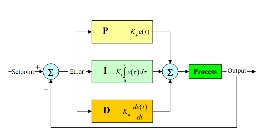
The PID controller algorithm involves three separate constant parameters, and is accordingly sometimes called three-term control:
- the proportional ( P)
- the integral (I)
- the derivative (D)
Simply put, these values can be interpreted in terms of time: P depends on the present error, I on the accumulation of past errors, and D is a prediction of future errors, based on current rate of change.The weighted sum of these three actions is used to adjust the process via a control element such as the position of a control valve, a damper, or the power supplied to a heating element.
Terminology:
The basic terminology that one would require to understand PID are:
- Error - The error is the amount at which a device isn’t doing something right. For example, suppose the robot is located at x=5 but it should be at x=7, then the error is 2.
- Proportional (P) - The proportional term is directly proportional to the error at present.
- Integral (I) - The integral term depends on the cumulative error made over a period of time (t).
- Derivative (D) - The derivative term depends rate of change of error.
- Constant (factor)- Each term (P, I, D) will need to be tweaked in the code. Hence,they are included in the code by multiplying with respective constants.
- P-Factor (Kp) - A constant value used to increase or decrease the impact of Proportional
- I-Factor (Ki) - A constant value used to increase or decrease the impact of Integral
- D-Factor (Kd) - A constant value used to increase or decrease the impact of Derivative
Error measurement:
In order to measure the error from the set position, i.e. the centre we can use the weighted values method. Suppose we are using a 5 sensor array to take the position input of the robot. The input obtained can be weighted depending on the possible combinations of input. The weight values assigned would be such that the error in position is defined both exactly and relatively.
The full range of weighted values is shown below. We assign a numerical value to each one.
| Binary Value | Weighted Value |
|---|---|
| 00001 | 4 |
| 00011 | 3 |
| 00010 | 2 |
| 00110 | 1 |
| 00100 | 0 |
| 01100 | -1 |
| 01000 | -2 |
| 11000 | -3 |
| 10000 | -4 |
| 00000 | -5 or 5 (depending on the previous value) |
The range of possible values for the measured position is -5 to 5. We will measure the position of the robot over the line several times a second and use these value to determine Proportional, Integral and Derivative values.
The Three Terms Explained:
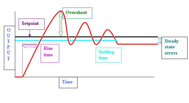
1.Proportional term:
The proportional term produces an output value that is proportional to the current error value. In simple terms, the more the error, the more the output value thus the further the setpoint is achieved (but beware of overshoot and instability). The proportional response can be adjusted by multiplying the error by a constant Kp, called the proportional gain.
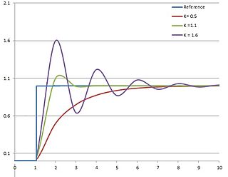
Plot of PV vs time, for three values of Kp (Ki and Kd held constant)
The proportional term is given by: Pout = Kp*e(t)
A high proportional gain results in a large change in the output for a given change in the error. If the proportional gain is too high, the system can become unstable (see diagram). In contrast, a small gain results in a small output response to a large input error, and a less responsive or less sensitive controller. If the proportional gain is too low, the control action may be too small when responding to system disturbances. Tuning theory and industrial practice indicate that the proportional term should contribute the bulk of the output change.
2.Integral term:
The contribution from the integral term is proportional to both the magnitude of the error and the duration of the error. The integral in a PID controller is the sum of the instantaneous error over time and gives the accumulated offset (steady state error) that should have been corrected previously. The accumulated error is then multiplied by the integral gain (Ki) and added to the controller output.
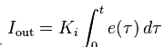
The integral term accelerates the movement of the process towards setpoint and eliminates the residual steady-state error that occurs with a pure proportional controller. However, since the integral term responds to accumulated errors from the past, it can cause the present value to overshoot the setpoint value (see diagram).

Plot of PV vs time, for three values of Ki (Kp and Kd held constant)
The main purpose of the integral term is to eliminate the steady state error. In the normal case there is going to be a small steady state error and the integral is mainly used to eliminate this error. It’s however true that when the error gets to 0 the integral will still be positive and will make you overshoot. Then after overshoot the integral will start to go down again. This is the negative effect of the integral term. So there is always the trade-off and you have to tune the PID controller to make sure that the overshoot is as small as possible and that the steady state error is minimized.
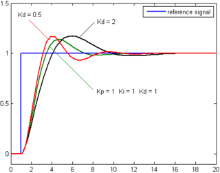
3.Derivative term:
The derivative of the process error is calculated by determining the slope of the error over time and multiplying this rate of change by the derivative gain Kd. The magnitude of the contribution of the derivative term to the overall control action is termed the derivative gain, Kd. The derivative term is given by: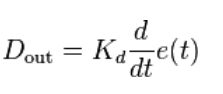
Derivative action predicts system behavior and thus improves settling time and stability of the system. An ideal derivative is not causal, meaning that it is very sensitive and can vary abruptly even with a small noise, so implementations of PID controllers include an additional low pass filtering for the derivative term, to limit the high frequency gain and noise. Derivative action is seldom used in practice though - by one estimate in only 20% of deployed controller - because of its variable impact on system stability in real-world applications. A PID controller without the Derivative term is called a PI controller.
The derivative term helps to minimize the overshoot in the system.
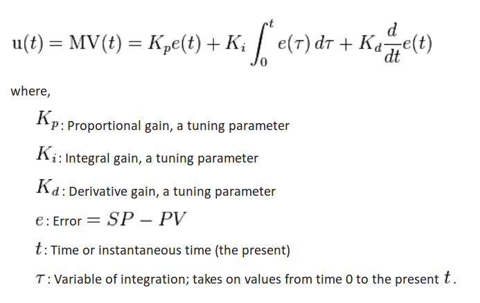
Final Expression:
The PID control scheme is named after its three correcting terms, whose sum constitutes the manipulated variable (MV). The proportional, integral, and derivative terms are summed to calculate the output of the PID controller. Defining as the controller output, the final form of the PID algorithm is:
Flowchart of the algorithm:
Consider an Example:
Lets assume you are driving down the road and trying to keep a set distance X behind the car in front of you.
Proportional Term : If you are following the car at X distance and you start to get further away from it, the error increases and you proportionally accelerate to close the gap back to X. If you accelerate too much you will overshoot X, making the distance now smaller than X so you need to slow down(negative error so negative acceleration) in order to get back to X. If you slow down too much you will pass X again and will need to accelerate to get back to X. This will continue if your proportional acceleration is not correct, this is the oscillation you see while tuning. The Proportional value controls how much effort is applied to correct the error.
Integral Term: The integral helps you regain the X distance again and maintain it a lot more accurately. It takes into account all the errors and cumulates them. If you are lagging behind the car, the error will be positive and it will drive you forward and vice versa. The integral in our example would be you returning to exactly X distance and maintaining it a lot smoother than just proportionally accelerating and decelerating. If your car is at X and say a speed bump makes you slow down, the integral will try return the car to X, whereas if you only had proportional it would only compensate with a proportional response and never actually hit the X perfectly. The integral is not perfect though and if not tuned well, it will slowly drift off of the X mark.
Derivative Term: The derivative is used to eliminate an accumulated error on the integral. Being a derivative term, it acts on the instantaneous change in error and helps smoothen situations like the arrival of a speed bump or sudden changes in error. It may also introduce oscillations as it is very noise sensitive. In our example this would be you noticing X distance growing ever so slightly and preventing the gap from getting any bigger. The derivative further prevents drift off the X mark. The derivative is only found on few controllers because of its noise prone nature, and is not entirely necessary. It does help keep the car stable if tuned well.
Manual tuning:
If the system must remain online, one tuning method is to first set Ki and Kd values to zero. Increase the Kp until the output of the loop oscillates, then the Kp should be set to approximately half of that value for a “quarter amplitude decay” type response. Then increase Ki until any offset is corrected in sufficient time for the process. However, too much Ki will cause instability. Finally, increase Kd, if required, until the loop is acceptably quick to reach its reference after a load disturbance. However, too much Kd will cause excessive response and overshoot. A fast PID loop tuning usually overshoots slightly to reach the setpoint more quickly; however, some systems cannot accept overshoot, in which case an over-damped closed-loop system is required, which will require a Kp setting significantly less than half that of the Kp setting that was causing oscillation.
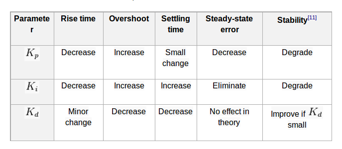
Effects of varying PID parameters (Kp,Ki,Kd) on the unit step response of a system.
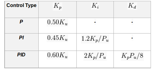
Ziegler–Nichols method:
Another heuristic tuning method is formally known as the Ziegler–Nichols method, introduced by John G. Ziegler and Nathaniel B. Nichols in the 1940s. As in the method above, the and gains are first set to zero. The proportional gain is increased until it reaches the ultimate gain, , at which the output of the loop starts to oscillate. and the oscillation period are used to set the gains as shown:
Pseudo Code:
Here is a simple loop that implements the PID control:
start:
error = (target_position) - (theoretical_position)
integral = integral + (error*dt)
derivative = ((error) - (previous_error))/dt
output = (Kp*error) + (Ki*integral) + (Kd*derivative)
previous_error = error
wait (dt)
goto start
Conclusion:
A PID controller relies only on the measured process variable, not on knowledge of the underlying process, making it a broadly useful controller. By tuning the three parameters in the PID controller algorithm, the controller can provide control action designed for specific process requirements. The response of the controller can be described in terms of the responsiveness of the controller to an error, the degree to which the controller overshoots the setpoint, and the degree of system oscillation. Note that the use of the PID algorithm for control does not guarantee optimal control of the system or system stability. Some applications may require using only one or two actions to provide the appropriate system control. This is achieved by setting the other parameters to zero. A PID controller will be called a PI, PD, P or I controller in the absence of the respective control actions. PI controllers are fairly common, since derivative action is sensitive to measurement noise, whereas the absence of an integral term may prevent the system from reaching its target value due to the control action.