Introduction
In Image processing, blob detection refers to modules that are aimed at detecting points and/or regions in the image that differ in properties like brightness or color compared to the surrounding.There are several motivations for studying and developing blob detectors. One main reason is to provide complementary information about regions, which is not obtained from edge detectors or corner detectors. It is used to obtain regions of interest for further processing. These regions could signal the presence of objects or parts of objects in the image domain with application to object recognition and/or object tracking.
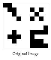
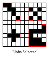
Blob detection is usually done after colour detection and noise reduction to finally find the required object from the image. A lot of unimportant blobs of the required color may be present in the picture and also we need the details of the blob like the blob centre, blob corners and all for which it is required that we know the exact coordinates of all the pixels in which the required blob is present in.
Algorithm- Recursive
The algorithm is simply going to count the number of pixels in the blob. This could easily be extended to actually collect the pixel locations to create a region. Keep in mind that in this example black pixels are “on” and white pixels are “off”. The basic idea is as follows:
1. To initialize, create a copy of the image, which will be altered to mark the progress of the algorithm.
2. Base Cases
a. If a pixel is off, return zero
b. If a pixel is out of bounds, return zero
3.Recursive Case
a. If a pixel is on
i. Turn off the current pixel
ii. Return 1 plus the sum of all 8 surrounding pixels.
And that’s the entire algorithm.
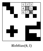
AN EXAMPLE: BlobSize(6,1)
An example might help to clear up any confusion. Let’s get the size of the blob located at pixel (6, 1). The following image is a visual representation of what the algorithm is going to do in the first two recursive calls.
 !{:.img-responsive}
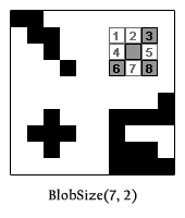
Assume our function is BlobSize(x as Integer, y as Integer) and returns an Integer (the number of pixels in the blob), and we are calling BlobSize(6, 1). We go back to the algorithm: step 1, this pixel is on and it is within the boundaries of the image, so we are not at a base case – skip to step 2. Step 2, the pixel is on, so turn it off and then return 1 + the sum of all surrounding pixels, that is:
Return _
BlobSize(5, 0) + BlobSize(6, 0) + BlobSize(7, 0) + _
BlobSize(5, 1) + 1 + BlobSize(7, 1) + _
BlobSize(5, 2) + BlobSize(6, 2) + BlobSize(7, 2)
Notice how each term in the return statement corresponds to a pixel from the 3×3 box in the image above (the 1 being the current pixel). The results from pixels 1, 2, 3, 4, 5, 6, and 7 will all be base cases and return 0 since they are off. But notice that pixel 8 is another recursive case, where it’s surrounding 8 pixels will be tested and the blob will expand. This function will ultimately return 5.
THE PROBLEM
Here is a comparison of the blob size (n) to the number of recursive calls (r):
n | r
-————–
5 | 41
6 | 49
13 | 105
1125 | 9001
1350 | 10801
2925 | 23401
The performance of this algorithm is 8n + 1 or O(n) in Big O notation. This causes a problem because the algorithm is recursive. The problem occurs for larger values of n.
The system runs out of stack space and you can get a StackOverflowException on larger n values.
Algorithm - Iteration
CONNECTED COMPONENT LABELLING
A graph, containing vertices and connecting edges, is constructed from relevant input data. The vertices contain information required by the comparison heuristic, while the edges indicate connected ‘neighbors’. An algorithm traverses the graph, labeling the vertices based on the connectivity and relative values of their neighbors. Connectivity is determined by the medium; image graphs, for example, can be 4-connected or 8-connected.
Following the labeling stage, the graph may be partitioned into subsets, after which the original information can be recovered and processed .
This algorithm makes two passes over the image one pass to record equivalences and assign temporary labels and the second to replace each temporary label by the label of its equivalence class.
Connectivity checks are carried out by checking the labels of pixels that are North-East, North, North-West and West of the current pixel (assuming 8-connectivity). 4-connectivity uses only North and West neighbors of the current pixel. The following conditions are checked to determine the value of the label to be assigned to the current pixel (4-connectivity is assumed)
Conditions to check:
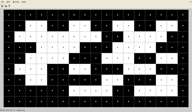
The array from which connected regions are to be extracted is given below
- Does the pixel to the left (West) have the same value?
- Yes - We are in the same region. Assign the same label to the current pixel
- No - Check next condition
- Do the pixels to the North and West of the current pixel have the same value but not the same label?
- Yes - We know that the North and West pixels belong to the same region and must be merged. Assign the current pixel the minimum of the North and West labels, and record their equivalence relationship
- No - Check next condition
- Yes - Assign the label of the North pixel to the current pixel
- No - Check next condition
- Yes - Create a new label id and assign it to the current pixel
- Does the pixel to the left (West) have a different value and the one to the North the same value?
- Do the pixel’s North and West neighbors have different pixel values?
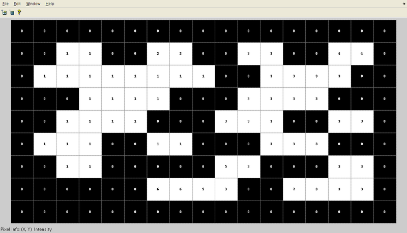
After the first pass, the following labels are generated. Note that a total of 7 labels are generated in accordance with the conditions highlighted above.
The label equivalence relationships generated are:
Set ID
Equivalent Labels
1
1,2
2
1,2
3
3,4,5,6,7
4
3,4,5,6,7
5
3,4,5,6,7
6
3,4,5,6,7
7
3,4,5,6,7
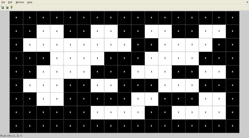
Array generated after the merging of labels is carried out. Here, the label value that was the smallest for a given region “floods” throughout the connected region and gives two distinct labels, and hence two distinct labels.
The algorithm continues this way, and creates new region labels whenever necessary. The key to a fast algorithm, however, is how this merging is done. This algorithm uses the union-find data structure which provides excellent performance for keeping track of equivalence relationships.Union-find essentially stores labels which correspond to the same blob in a disjoint-set data structure, making it easy to remember the equivalence of two labels by the use of an interface method E.g.: findSet(l). findSet(l) returns the minimum label value that is equivalent to the function argument ‘l’.
Once the initial labeling and equivalence recording is completed, the second pass merely replaces each pixel label with its equivalent disjoint-set representative element.
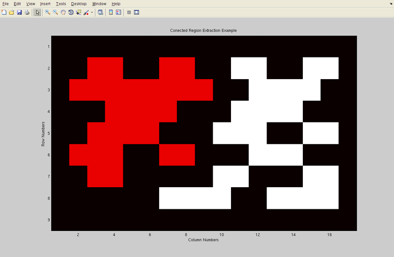
Final result in color to clearly see two different regions that have been found in the array.
PROGRAM