Introduction
In statistics, a histogram is a graphical representation of the distribution of data. It is an estimate of the probability distribution of a continuous variable. A histogram is a representation of tabulated frequencies, shown as adjacent rectangles, erected over discrete intervals (bins), with an area equal to the frequency of the observations in the interval. The height of a rectangle is also equal to the frequency density of the interval, i.e., the frequency divided by the width of the interval. The total area of the histogram is equal to the number of data. A histogram may also be normalized displaying relative frequencies. It then shows the proportion of cases that fall into each of several categories, with the total area equaling 1. The categories are usually specified as consecutive, non-overlapping intervals of a variable. The categories (intervals) must be adjacent, and often are chosen to be of the same size. The rectangles of a histogram are drawn so that they touch each other to indicate that the original variable is continuous.
Why do we use Histograms?
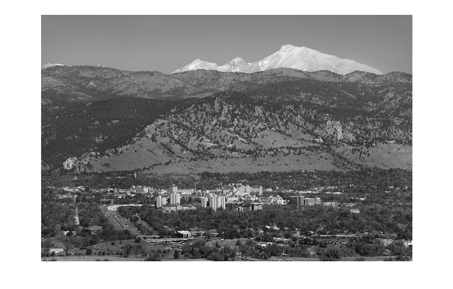
Histograms are generally used to find the threshold level of an image to perform further image enhancing operations. For example, the median level of an histogram is often used as a threshold to convert a grayscale image to binary.
Generating Histograms
The histogram of a digital image with L total possible intensity levels in the range [0,G] is defined as the discrete function
h(r)=n
where r is the kth intensity level in the interval [0,G] and n is the number of pixels in the image whose intensity level is r. The value of G is 255 for images of class uint8, 65535 for images of class uint16, and 1 for images of class double.
Often we work with normalised histograms, which are obtained by dividing h by the total number of pixels in the image. We recognise that this is an estimate of the probability of occurrence of intensity level r.
The core function for dealing with histograms in the IPT is imhist.
where f is the input image, b is the number of bins used in forming the histogram ( default is 256) and h is the histogram.
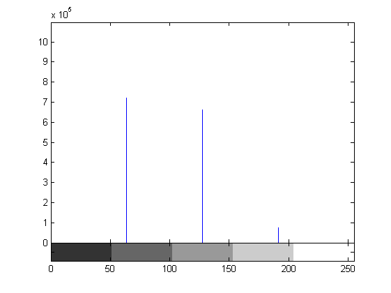
For example if we are working with uint8 images and we let b=2 then the intensity scale is divided into two ranges 0-127, and 128 to 255. The resulting histogram has two values h(1)) equal to number of pixels in (0,127) and h(2) having number of pixes between (128, 255). Normalised histogram is obtained by
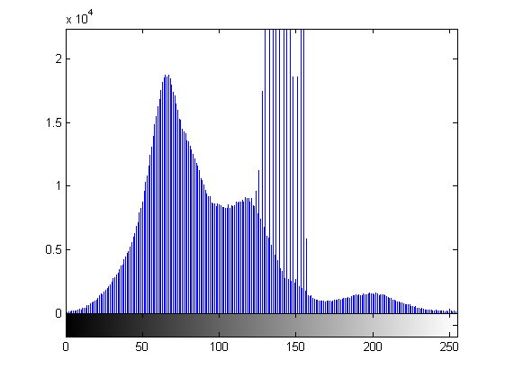
The simplest way to plot its histogram is to use imhist with no output specified.
This would produce
whereas
produces
However there are many other ways to plot histograms like for example, using bar graphs.
v is the row vector containing plots to be plotted, horz is a vector of same dimension as v containing the increments of the horizontal scale and width is number between 0 and 1. Default value of width is 0.8. At 1 the bars touch and at 0 they are simply vertical lines.
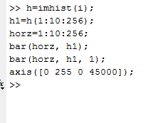
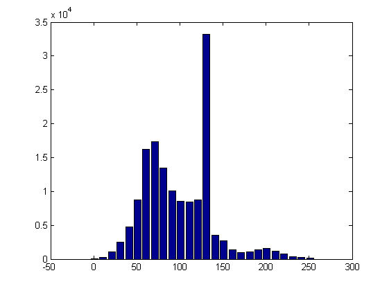

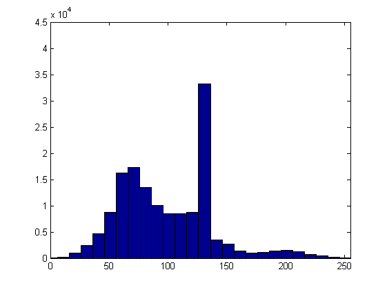
The first histogram has the default width value ( 0.8) while the second has a width of 1. The third histogram has a longer vertical axis and the horizontal axis set to 256 which can be done by the axis command as seen in the code above.
Other ways to plot graphs are stem and plot commands.
Histogram Equalisation
The function histeq attempts to distribute the levels so that they will approximate to a flat histogram. This leads to a higher dynamic range(HDR) with an increased contrast.
where f is the input image and nlev is the number of intensity levels specified for output image. Default value for nlev is 64 unlike the imhist function. Usually we use the maximum number of possible levels for nlev because this produces a true implementation of the histogram equalisation method.

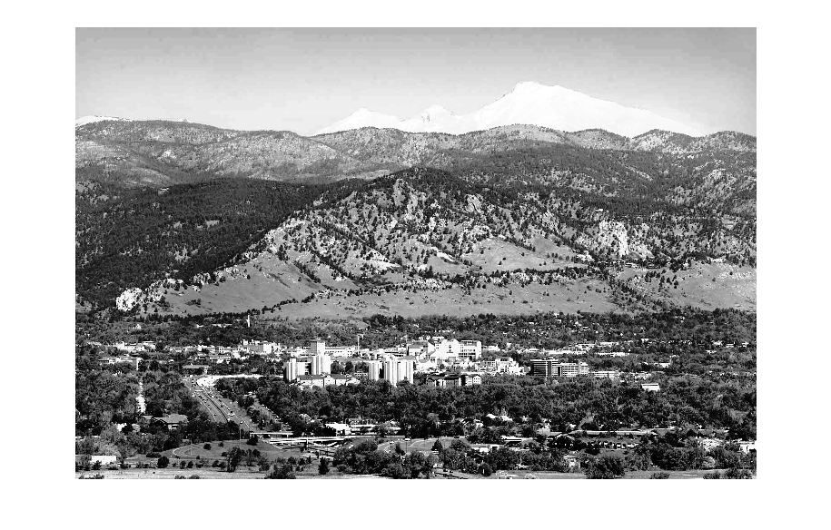
HIstograms of the two images

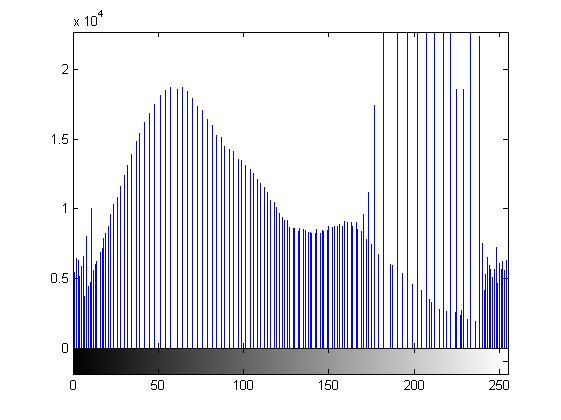
As we can see, the second histogram is much more spread out over the axis.